Self-organization during development. Diverse skin patterns form on zebrafish due to the interactions of pigment cells. (A) Wild-type zebrafish feature dark stripes and light interstripes (4, 11), while mutant patterns that form because a particular cell type is missing have altered, more variable patterns. (B) The nacre mutant (encoding mitfa) (9, 12) has an enlarged central orange region flanked by blue patches. (C) Pfeffer (encoding csf1rA) (9, 10, 13) is characterized by messy spots arranged horizontally (11). (D) Shady (encoding ltk) (11, 14) often features smooth black spots roughly arranged in stripes. Reproduced from ref. 11, which is licensed under CC BY 3.0. (E) Pigment cells extend long legs (measuring up to half a stripe width in distance) toward interstripe cells for communication (26). Reproduced from ref. 26, which is licensed under CC BY 3.0. (F–I) The agent-based model (20) replicates zebrafish patterns in silico. (Red scale bar, 500 μm throughout this paper.) The central light interstripe is labeled X0, and the next two interstripes are called X1V and X1D (11). (J) Rules for agent behavior in the model (20) depend on the cells in short-range disks and a long-range annulus. Reproduced from ref. 20, which is licensed under CC BY 4.0. (K) Summary of the main pigment cells involved in patterning. Interstripes consist of orange dense xanthophores and silver dense iridophores, and stripes contain yellow loose xanthophores, blue loose iridophores, and black melanophores.

Illustration of persistent homology applied to coordinate data. (A and B) Noisy data sampled from a figure-eight shape (A) and corresponding manifold expansions (B).

Illustration of our topological techniques applied to zebrafish patterns. (A) Boundary conditions are periodic in the horizontal direction, so stripes and interstripes are viewed as loops from a topological perspective. (B) We count interstripes and measure stripe width using persistent homology. We show manifold expansions of the locations of Xd cells by considering balls of growing radius r centered at the location Xid of each cell. When r=r1, the radius of the balls is about half the maximum distance between neighboring Xd cells Δxx. At this point, three interstripes have formed, but the number of loops is larger than the true number of interstripes due to gaps between cells, highlighted by red arrows (β0=3 and β1>3). As r increases to r2, the noisy loops die off, leaving only three loops (β0=3 and β1=3). The long persistence of three loops corresponds to the true presence of three interstripes. As r increases further to r4, the manifold collapses to a single connected component (β0=1 and β1=1). The difference between the ball radius at which this collapse occurs (r4) and the ball radius at which three loops appear (r1) approximates half the maximum width of black stripes. (C) By combining TDA with clustering methods, we automatically detect interstripe boundaries and measure their curviness; we show the percentage of increase in arc length distance (ALD) of these boundaries (traced out in red) relative to perfectly straight stripes here. (D) We describe spotted phenotypes by combining persistent homology, clustering methods, and principal component analysis. We use β0 to quantify the number of spots. As an example, we show the spot size and spot roundness for two nacre spots.

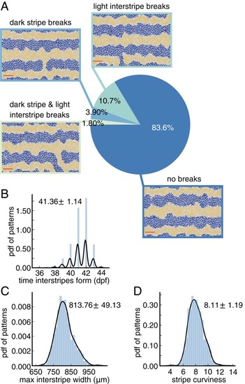
Baseline quantification of wild-type patterns. All measurements are based on 1,000 simulations of the model (20) under the default parameter regime. (A) We use persistent homology to detect the presence of breaks in stripes and interstripes. (Following the example in ref. 20, we do not count breaks in the dark stripes along the top and bottom boundaries of the domain.) The domain captures about one-third of the fish body (20). (B) Distribution of times at which interstripes X1D and X1V (Fig. 1F) begin to form. (C) Distribution of maximum interstripe width. (D) Distribution of stripe curviness (also see Fig. 3C). In B–D, we display histograms of in silico data and kernel density estimator (KDE) curves with a Gaussian kernel in black; the mean plus/minus the SD is shown in each plot for the data.

Baseline study of mutant patterns to extract quantifiable features. All measurements are based on 1,000 simulations of the model (20) (for each mutant) under the default parameters. Histograms show distributions for (A) the number of spots, (B) spot size, (C) spot roundness, (D) variance in spot spacing, and (E) X0 interstripe width (Fig. 1G). We overlay KDE curves with a Gaussian kernel on the histograms; the mean plus/minus the SD is shown in each plot for the data.

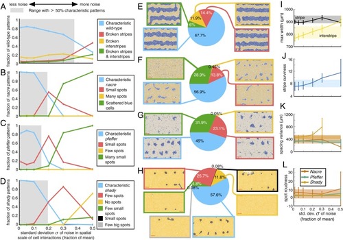
Quantitative study of how stochasticity in cell interactions affects wild-type and mutant zebrafish patterns. For each value of σ∈{0.01,0.05,0.1,0.2,0.3,0.5}, where σ times the default length scale is the SD of the noise that we include in the size of cellular interaction neighborhoods, we analyze 1,000 simulations for wild type and each mutant. (A–H) Summary of the patterns that emerge under stochasticity, as detected using our methods for (A and E) wild type, (B and F) nacre, (C and G) pfeffer, and (D and H) shady. In A–D, we highlight the range of σ values that retain at least 50% characteristic patterns under noise in gray. (We define “characteristic” for wild type as patterns having three unbroken interstripes and two unbroken stripes, and we define characteristic for mutants as patterns with spot size and spot number that fall within the baseline distributions in Fig. 5 A and B.) (I and J) Mean maximum stripe/interstripe width (I) and mean stripe curviness (J) for wild type for different noise strengths. (K and L) Spot spacing variance (K) and spot roundness (L) for mutants under different noise strengths. In I–L, the bars indicate SD and the shaded regions give the characteristic values (the mean ±1 SD) for the associated measurements from our default studies. Also see SI Appendix, Tables S2–S5.

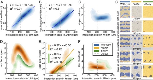
Quantifying in silico pattern dependence on the spatial scale of long-range cellular interactions involved in M birth. (A–F) Kernel density estimates for (A and B) maximum stripe and interstripe width for wild type, (C) wild-type stripe curviness, (D) number of spots for pfeffer and shady, (E) median spot size for the mutants, and (F) pfeffer and shady spot roundness as a function of the inner radius of the Ωlong neighborhood in Eq. 1. Measurements in A–F are based on 100 simulations of the model (20) (for wild type, pfeffer, and nacre, respectively) for each inner radius R of Ωlong in [1] considered. (We consider R from 10 to 400 μm in increments of 25 μm.) All other model parameters (including the width of the Ωlong annulus in Eq. 1 and the long-range annulus scale in all other model rules) remain at their default values. In A, B, and E we show linear regression models for their corresponding values, along with the R2 goodness-of-fit scores. (G) Example wild-type, pfeffer, and shady patterns for different parameter values [the patterns generated by the model (20) under the default parameter—210 μm—are noted in gray].