The PIV algorithm, and comparison between two shift estimation methods. (a) Sub-regions of the frame pairs are cross-correlated in time, yielding a matrix of the cross-correlation result, the peak of which then indicates the most likely motion of particle image between the two frames. Peak detection is then followed by subpixel interpolation of the peak and certain criteria tests probing the validity of the measurement, details in [25]. In case of correlation-averaging, each result IW pair matching from the same phase is averaged before peak fitting is executed. (b) shows the standard analysis based on direct cross correlation, while (c) illustrates our substitution of the sum of absolute differences metric in the cross-correlation stage of the analysis. Notice that the calculated flow in (b) is biased towards high intensities and produces vectors which appear to be pointing inwards, towards the center of the blood vessel. The same parameters were used in the PIV algorithm for both analyses.

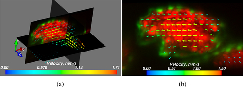
3D flow reconstruction using 2D flow data in the zebrafish heart (walls expressing flk1:GFP and RBCs expressing gata:DsRed). (a) 3D cut-plane image of blood flow in a ∼3 dpf zebrafish heart. Peak flow vectors (corresponding to the high end of the colorbar) are plotted, but not visible in this orientation. For the most part of the heart the calculated flow field is smooth. The erroneous areas mostly correspond to positions where the flow is out-of-plane. The flow measurements are reliable as long as the plane of the flow is reasonably well-aligned with the imaging plane (in-plane motion dominates over out-of-plane motion). The sample mounting in SPIM allows many sample orientation options, however, the geometry of the heart often determines a preferred orientation for flow imaging. (b) Close up of the xy plane of (a). Visualization 1 in the supplementary material also shows the flow in the heart, over the full heartbeat. Visualization 2 further illustrates the depth-resolved flow results at a single phase. The square root of velocity magnitudes is displayed to better demonstrate the dynamic range. Visualized using Mayavi [32].