Cellular-Resolution Imaging of the Entire Larval Zebrafish CNS with SPED Light Sheet Microscopy

(A and B) Volume renderings of 10 dpf Tg(elavl3:H2B-GCaMP6s) zebrafish larvae imaged with 4×/0.28NA (A) and 10×/0.25NA (B) objectives demonstrate the large field of view of SPED microscopy, while maintaining cellular resolution. Cyan and magenta boxes provide magnified views. (A) Image volumes of 10 consecutive time points were collapsed into one volume by taking the maximum values voxel-wise across the recording duration. The bounding box size is 0.75 mm × 2.99 mm × 0.48 mm. (B) Image volumes of 7 consecutive time points were collapsed into one volume by taking the maximum values voxel-wise across the recording duration. The bounding box size is 0.65 mm × 1.20 mm × 0.30 mm. See Movies S3 and S4 for detailed 3-dimensional rendering and Figure S5 for comparison of raw and deconvolved data.

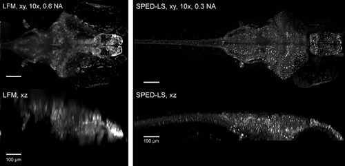
Comparing Resolution of LFM and SPED Light Sheet Methods

Three-dimensional volumes were acquired from a 10 dpf Tg(elavl3:H2B-GCaMP6s) zebrafish larva with LFM and SPED light sheet microscopy, using 10×/0.6NA (water immersion, Olympus) objective with 500 ms exposure and 10×/0.3NA (air, Olympus) objective with 460 ms exposure, respectively. SPED light sheet images in Figure 6B were acquired with less than 100 ms exposure/volume, still yielding cellular resolution. Scale bars, 100 µm.

Rapid Cellular-Resolution Functional Mapping of the Entire Larval Zebrafish Nervous System

(A–C) The camera-frame-rate limited volumetric imaging speed of SPED light sheet is demonstrated by performing rapid cellular-resolution functional mapping of the nervous system of 10 dpf Tg(elavl3:H2B-GCaMP6s) zebrafish larvae. Three smaller ROIs of the camera frame were used to image: (A) the entire nervous system with a 4×/0.28 NA objective at 6.23 volumes per second (3 mm × 0.5 mm × 0.2 mm, 39 z slices), (B) the whole brain with a 4×/0.28NA objective at 12 volumes per second (0.9 mm × 0.4 mm × 0.2 mm, 40 z slices), and (C) the whole brain and anterior spinal cord with a 10×/0.25NA objective at 4.14 volumes per second (1.2 mm × 0.43 mm × 0.2 mm, 39 z slices). The maximum intensity projection images were generated from a collapsed 3D volume generated by voxel-wise standard deviation (SD) across the entire recording durations. Cellular resolution is demonstrated by several examples of activity traces (ΔF/F versus time) of neurons marked by colored arrows, and of neighboring cells shown in optical slices from respective volumes and their automated 3D segmentation. See Figure S6 for the top 99 example activity traces (ordered according to the variance across time) from the three datasets. Movies S5, S6, S7 exhibit the activity time series (ΔF/F versus time) of these datasets, and Movie S8 shows details of automated 3D segmentation.

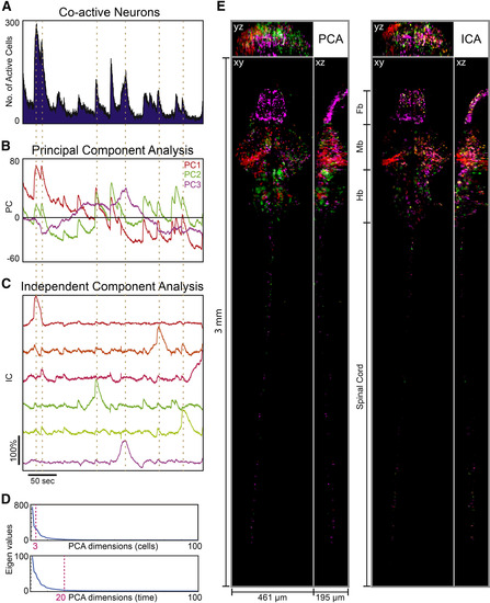
Population Analysis of Global Zebrafish CNS Activity Recorded by SPED Light Sheet Microscopy

Principal component analysis (PCA) and independent component analysis (ICA) were used to analyze the population dynamics of neurons spread across the entire zebrafish larval CNS. The dataset was acquired using a 4×/0.28 NA objective at 6.23 volumes/sec (as in Figure 6A). ΔF/F activity profiles of all cells were first filtered to identify active neurons by choosing a noise level corresponding to 5% false positive rate as the cutoff, followed by PCA and ICA; early time points that may represent nonspecific responses to initial laser illumination were excluded from analysis.

(A) Number of co-active neurons as a function of time across the recording duration.

(B) Temporal traces of top three principal components (PC) shown in red, green and magenta respectively. y axis represents arbitrary units in PCA space.

(C) Temporal traces of 6 recovered independent components (IC) out of 10 (filtered to retain traces in which the sum of minimum and maximum values was greater than zero); units are arbitrary. The dotted lines across panels indicate peaks in the ICs that correspond to the peaks in PCA and cellular activity.

(D) Eigenvalues for the top 100 dimensions of cellular (top) and time points (bottom) principal components. Dashed lines mark the top 3 cellular and the top 20 temporal PCA dimensions, which were used in (B) and for data “whitening” before ICA (methods) in (C).

(E) Spatial plots of each PC coefficient (absolute value) and each IC (absolute value) were generated to visualize the locations and identities of the neurons associated with each component.

Different components were combined into multi-color images (each color corresponding to coloring of the temporal traces in B and C) after scaling for contrast. Images shown are maximum intensity projections through x, y or z. Fb, Forebrain; Mb, midbrain, Hb, Hindbrain.

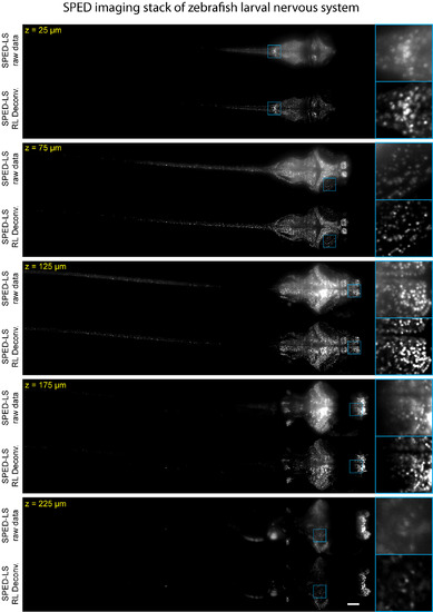
Comparison of Raw and Deconvolved SPED Light Sheet Data Stack, Related to Figure 4

A consecutive series of optical sections (50 µm thick) is shown to demonstrate image quality enhancement after deconvolution. Data were acquired from a 10 dpf Tg(elavl3:H2B-GCaMP6s) zebrafish larva using 4×/0.28NA detection objective. Image volumes of 10 consecutive time points (arbitrarily chosen number to increase labeled cell count) were combined into one volume by taking the maximum values of the voxels across the time points. Detailed volume rendering of the image stack is shown in Figure 3A and Movie S3. Scale bar, 100 µm.

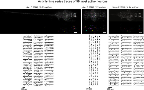
Neuronal Activity Time Series across the Intact Nervous System, Related to Figure 6

Neuronal activity traces (ΔF/F) are shown for top 99 most active neurons in the larval zebrafish nervous system (assessed by variance across the entire recording duration), imaged using 4×/0.28 NA objective at 6.23 volumes/second (3 mm × 0.5 mm × 0.2 mm, 39 z slices), 4×/0.28 NA objective at 12 volumes per second (0.9 mm × 0.4 mm × 0.2 mm, 40 z slices) and 10×/0.25 NA objective at 4.14 volumes per second (1.2 mm × 0.43 mm × 0.2 mm, 39 z slices). Spatial distribution of identified cells is overlaid on the maximum intensity projection image of voxel-wise SD across the entire recording duration. Scale bars, 100 µm.