Fig. 6

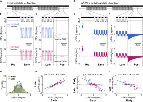
The model is generalizable across individuals

(A and D) The stimulus image pattern and the stimulus velocity are shown as horizontal bars and lines, respectively.

(B and C) The simulated slow-phase velocity (SPV) of Figure 4A (color line) is compared to the median ± median absolute deviation of simulations from all 29 subjects (black line with gray shadow).

(E and F) The difference of SPVs between the individual simulation (color line in B and C) and the population median (black line in B and C). Dashed lines extend from (D) to (E and F) illustrate the time windows for further analyses in (G–J).

(G) The ΔSPV probability distribution of 29 fish during the early and late periods. Two lines demonstrate the fit of distributions with Gaussian function.

(H) The late ΔSPV plotted over the early ΔSPV. The slope of linear regression line (solid line) is significantly smaller than 1 (p = 5.58e-19; interactive analysis of covariance) and the slope of the dashed line (temporally shuffled data; p = 1.94e-18; interactive analysis of covariance).

(I) The changes in ΔSPV across stimulus phases (late ΔSPV – early ΔSPV, ΔΔSPV) plotted over the early ΔSPV. The slope of linear regression line (solid line) is significantly lower than the dashed line (temporally shuffled data; p = 1.94e-18; interactive analysis of covariance).

(J) The changes of the eye movements in the dark before and after optokinetic nystagmus (post-ΔSPV – pre-ΔSPV, ΔΔSPV) plotted over the early ΔSPV. Filled circles represent the data of the animal shown in (A–F).

(H and I) Black solid lines demonstrate the linear regression fit of simulated data. Considering the starting direction of alternating stimulation was randomized, we aligned the first stimulus direction as positive instead of left or right. Therefore, the plots show one eye started with a nasalward movement (blue trace) and another eye started with a temporalward movement (red trace). p, p values; Pearson correlation. R, correlation coefficients; Pearson correlation.