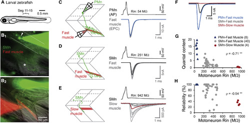
Motoneuron-Muscle Paired Recordings Reveal Differences in Strength and Reliability of Motoneuron Outputs

(A) Schematic of a 5 dpf larval zebrafish. Light gray shading marks the brain and spinal cord. Recordings were done at body segment 11–15.

(B) Experimental preparation for paired recordings on a secondary motoneuron (SMn) and a fast muscle cell, filled with Alexa Fluor 488 and 568, respectively.

(B1) Focal plane of the SMn cell body (arrowhead) and its main axon (asterisk). Dashed lines mark the boundaries of the spinal cord.

(B2) A more superficial focal plane with the motoneuron axonal projections and boutons that overlap with the recorded muscle cell.

(C–E) Schematics (left) and example traces (right) of whole-cell current-clamp recordings from a spinal motoneuron and whole-cell voltage-clamp recordings from a muscle cell (C, primary motoneuron [PMn]-fast muscle; D, SMn-fast muscle; E, SMn-slow muscle). The averaged waveform of motoneuron action potentials (APs; n = 10; firing at 1 Hz) is shown in black. The input resistance of the recorded motoneuron is indicated. Individual evoked endplate currents (EPCs; n = 10; gray) and their averaged waveform (colored) are temporally aligned to the peak of motoneuron action potentials to show the variability in amplitude. Note the different scales for EPC amplitude. The round-shaped EPCs in the example SMn-slow muscle recording are filtered inputs from neighboring muscle cells electrically coupled to the recorded muscle cell [17]. The red trace represents the averaged waveform of all ten individual current responses in (E), including responses to direct synaptic inputs (fast responses), electrically coupled inputs (slow responses), and failures.

(F) Averaged EPC waveforms of the three example recordings in (C)–(E) are temporally aligned to the peak of motoneuron action potentials.

(G) Quantal content of motoneuron outputs versus input resistance (Rin) of motoneurons. The number of recordings is indicated in parentheses. ^∗∗p < 0.01 following Spearman’s rank test (ρ is shown).

(H) Reliability of motoneuron action potentials eliciting EPCs versus motoneuron Rin. ^∗∗p < 0.01 following Spearman’s rank test (ρ).

See also Figure S1.

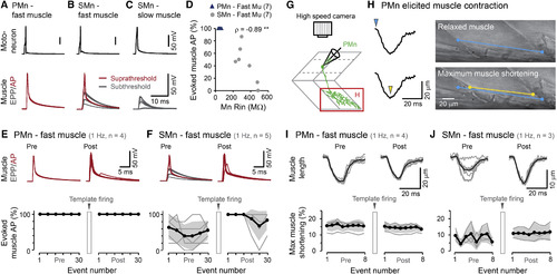
Secondary Motoneurons More Reliably Elicit Fast Muscle Action Potentials and Muscle Contractions after Repeated Motoneuron Firing with the Template Pattern

(A–C) Example traces of paired current-clamp recordings of a motoneuron and a muscle cell (A, PMn-fast muscle; B, SMn-fast muscle; C, SMn-slow muscle). Top: averaged waveform of motoneuron action potentials (n = 10). Bottom: voltage responses of muscle cells, temporally aligned to the peak of motoneuron action potentials (n = 10). Subthreshold endplate potentials (EPPs) are shown in gray; muscle action potentials are in red. Muscle voltage changes in (A)–(C) share the same scale.

(D) The reliability of motoneuron firing eliciting muscle action potentials versus motoneuron input resistance (Rin). ^∗∗p < 0.01 following Spearman’s rank test (ρ is shown).

(E and F) Muscle voltage change in response to 1 Hz, 30 s motoneuron firing before (Pre) and after (Post) repeated template firing. Templates 1 and 2 were used for PMn-fast muscle (E) and SMn-fast muscle (F) paired recordings, respectively. Top: example traces of the first ten muscle voltage responses temporally aligned to the peak of motoneuron action potentials. Bottom: group data for the ratio of motoneuron action potentials able to elicit muscle action potentials (5 s/five event bin; 1, suprathreshold; 0, subthreshold; gray lines, individual recordings; thicker black line with shading, mean ± SD).

(G) Experimental preparation for simultaneous patch recording of a motoneuron and video recording of elicited muscle contractions. The red rectangle marks the region for muscle length measurements in (H).

(H) Right: the blue and yellow dots mark the two ends of a fast muscle cell at its relaxed and maximally contracted state, respectively, during a PMn-elicited contraction. Left: the time course of muscle length change during the contraction with blue and yellow arrowheads indicating the relaxed state and maximum contraction, respectively.

(I and J) The amount of muscle shortening in response to 1 Hz, 8 s motoneuron firing (I, PMn; J, SMn) before (Pre) and after (Post) repeated template firing. Top: example traces of the muscle length time course (n = 8; gray lines) aligned temporally with their averaged waveform (black line). Bottom: group data showing the maximum muscle shortening, normalized to the original muscle length, in response to each motoneuron action potential (gray lines, individual recordings; thicker black line with shading, mean ± SD).

See also Figure S4 and Movies S1 and S2.