Figure 2.

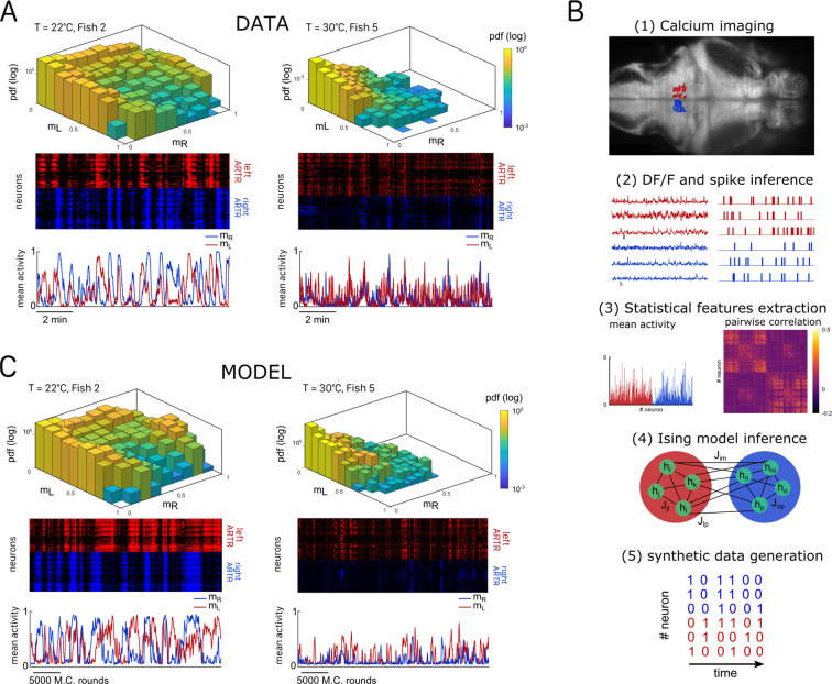
(A) (Top) Probability densities P(mL,mR), see Equation 2, of the activity state of the circuit (obtained from the spiking inference of the calcium data), in logarithmic scale, and for two different fish and water temperatures T = 20 and T = 30°C; Color encodes z-axis (same color bar for both). (Middle) 10-min-long raster plots of the activities of the left (red) and right (blue) subregions of the anterior rhombencephalic turning region (ARTR). (Bottom) Corresponding time traces of the mean activities mL and mR. (B) Processing pipeline for the inference of the Ising model. We first extract from the recorded fluorescence signals approximate spike trains using a Bayesian deconvolution algorithm (BSD). The activity of each neuron is then ‘0’ or ‘1.’ We then compute the mean activity and the pairwise covariance of the data, from which we infer the parameters hi and Jij of the Ising model. Finally, we can generate raster plot of activity using Monte Carlo sampling. (C) Same as (A) for the two corresponding inferred Ising models. The raster plots correspond to Monte Carlo-sampled activity, showing slow alternance between periods of high activity in the L/R regions. Here we show only two examples of a qualitative experimental vs. synthetic signals comparison. We provide in the supplementary materials the same comparison for every recording.