
|
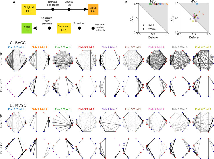
Figure 7.
(A) Description of the whole pipeline. Before running the GC analysis on the raw calcium transients (DF/F), the lag parameter must be chosen. Then, before running the GC analysis again, motion artifacts are corrected, the fluorescence is smoothed and a new threshold is calculated. (B) Comparison of WIC and WRC before and after applying the pipeline to the GC analyses. Points in the upper right triangle gray-shaded area represent the ratios that have increased in the final GC results. Each fish (n=9) is represented by a color, BVGC by circles and MVGC by triangles. Means are shown in black. We find that using our pipeline, WIC strongly increases and we can clear out the spurious contra-lateral links present in the original GC. WRC is not significantly improved: the recording frequency and GCaMP decay are likely too low and slow compared to the speed of rostro-caudal propagation of the information flow. (C) Network results before (top row) and after (bottom row) applying our pipeline for computing bivariate Granger causality (BVGC), for all fish. For consistency in the network representation and better ability to compare, we removed the uncharacteristically behaving neurons of the GC analysis before applying the pipeline. Note that more links are found on the side that was better in focus in the recording. (D) Same as (C) but for the multivariate Granger causality (MVGC).