CNMF with and without initial decimation to speed up CNMF.

(A) Real data summary image obtained as max-projection along time-axis. Squares indicate patches centered at suspected neurons. The three highlighted neurons are considered in the next panels. (B) Extracted shapes of the three neurons highlighted in (A) using the same color code. The upper row shows the result with initial temporal decimation by a factor of 30 and spatial decimation by 3×3, followed by five final iterations on the whole data. The algorithm ran for merely 1 s. The lower row shows the result without any decimation and running until convergence, yielding virtually identical results. (C) Extracted time traces without (thick black) and with initial iterations on decimated data (color as in A) overlap well after merely 1 s. (D) They overlap almost perfectly if the algorithm using decimation is run not only for 1 but 10 s.

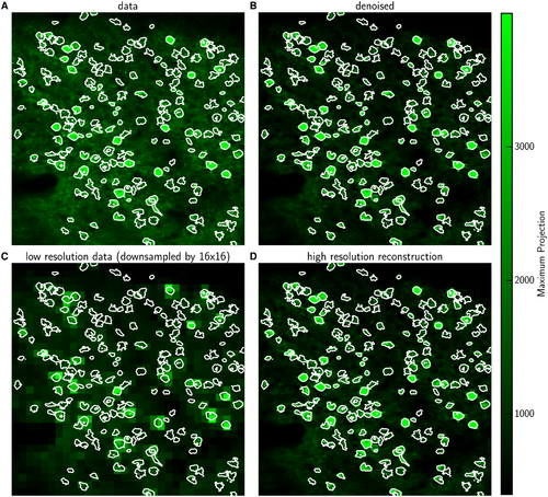
Previously identified shapes allow reconstruction at high spatial resolution based on low resolution imaging (best seen in S2 Video for full details).

(A) Max projection image of the raw data Y with identified ROIs, i.e. neurons or activity hotspots. Contour lines contain 90% of the energy of each neural shape. (B) Max projection image of the denoised estimate A₁ ⋅ C₁ (plus the estimated background). (C) Max projection image for data obtained at lower spatial resolution, Y_l; l = 16 here. (D) Reconstruction based on the low resolution data in (C) and previously identified shapes, A₁ ⋅ C_l. The reconstruction looks very similar to the denoised high-resolution data of (B). Note: contours in (B-D) are not recomputed in each panel, but rather are copied from (A), to aid comparison.

,p>Estimating neural shapes on small initial batch of the data.

(A) Shapes inferred on the full data (orange) or using only the first half (blue). Two apparently lost suspected ROIs (white arrows) are actually part of another neuron (blue arrow) (B) Average correlation (±SEM) between traces C_l obtained on decimated data and the reference C₁ obtained without any decimation. Similar results hold for median and IQR, but the resulting plot is too cluttered. (C) Comparing to simulated ground truth C^s. Traces were obtained on decimated data with reshuffled residuals, otherwise analogous to (B).

Interleaving improves accuracy of recovered C_l at low spatial resolution.

(A) Interleaving alternates between pixels corresponding to the cyan and orange grid. (B) Correlation between traces C_l obtained on decimated data and the reference C₁ obtained without any decimation. The average correlation (±SEM) decays faster without (cyan) than with interleaving (green). Similar results hold for median and IQR, but the resulting plot is too cluttered. (C) Comparing to simulated ground truth C^s. Traces were obtained on decimated data with reshuffled residuals, otherwise analogous to (B).