a Schematic outline of the reconstruction procedure. The global fields Y_E(t) and Y_I(t) constitute the inputs of the model in the HMF approximation (i). Different choices for the probability distributions P_E(k), P_I(k), and P(a) are iteratively tested in order to find the best match between the input fields and the reconstructed fields, as obtained by using the equations displayed in the red box (ii). b Outcome of the reconstruction procedure: the true probability distributions of a synthetic network are compared with those obtained with the proposed reconstruction method. A random network with N = 5000 is considered here. The fraction of inhibitory neurons is set to f_I = 0.05. The number of classes defined in the HMF approximation for the in-degree and the external current is L = 250 and M = 250 respectively. c Comparison between the true global fields and the ones obtained via the reconstructed distributions. The plot in the inset is a zoom in of a peak. D-E) Outputs of the reconstruction are compared with the true external current probability distribution P(a) and the true in-degree distribution P_E(k) for the excitatory neurons of the same network; the network is made of N = 1000 neurons of which a fraction f_I = 0.2 are inhibitors. In the HMF approximation one hundred classes have been defined for both the in-degree and external current, namely, L = 100 and M = 100. In D) the correct fraction of inhibitory neurons is taken into account, while in E) the inhibitory neuron effects are not considered

Main steps of experimental data elaboration. Every layer of the imaged 3D zebrafish brain is spatially downsampled, as shown in panel a in order to obtain signals from pixel ensembles of size comparable to a neuron (2 × 2 pixels). b Detrending for slow oscillations by subtraction of moving average. c Results of neurons selection for one of the layers: (i) raw data, (ii) selection of pixels with maximum value above a fixed threshold, and (iii) only pixels with skeweness larger than 0.4. At the end of the neurons selection procedure the number of identified neurons in the whole brain is about 5 ⋅ 10⁴. d Procedure to obtain the experimental raster plot starting from calcium fluorescence time series of the selected neurons. A spike is identified by its upwards threshold crossing time

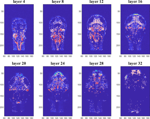
Detected neurons for eight different layers of the zebrafish brain. Colours represent the average cross-correlation of each neuron with all the others selected neurons of the brain

a The ISI is computed for both excitatory (red symbols, top panel) and inhibitory (purple symbols, bottom panel) neurons. The prediction based on the HMF approximation yields the continuous curves. Here N = 1000 and f_I = 0.2. b The relative error 〈ΔY_EE/Y_EE〉_t committed when using the approximation Eq. (15) is plotted for different values of f_I