
- Title
-
Adaptation mechanism of the adult zebrafish respiratory organ to endurance training
- Authors
- Messerli, M., Aaldijk, D., Haberthür, D., Röss, H., García-Poyatos, C., Sande-Melón, M., Khoma, O.Z., Wieland, F.A.M., Fark, S., Djonov, V.
- Source
- Full text @ PLoS One
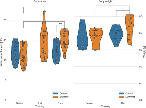
Left: max. achieved swimming speed by untrained and trained fish (n = 20 per group, except for swimmers at 5wk n = 19). Data for the control group at 3 weeks were not recorded. Significant differences are found for the swimmers in the performance before training compared to either 3 weeks (p = 0.00029) or 5 weeks of training (p = 7.8e-8). Controls and swimmers at 5 weeks also showed a significant difference in critical speed (p = 2.7e-6). All other combinations are not significant. Right: weight of all the fish was measured before and after 5 weeks of swimming (n = 10 for each group). Significant differences are found in the weight of the swimmers before and after training (p = 0.011) and between the control and swimmer group after training (p = 0.041). wk = week, *: p<0.05, ***: p<0.001, lines within the plots show the quartiles of the respective distributions. |
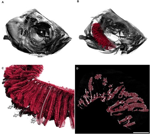
A: Fish head. The diameter of the whole eye (centre marked with a white asterisk) is approximately 0.83 mm. B: The delineated gills in red are shown inside the head of the fish, operculum removed, only right arches of the gills are shown. The gill arches lie within the branchial chamber. In this image, primary filaments are mainly pointing to the left of the image (back of fish). C: Detailed view of gills. Secondary filaments are seen as leaf-like structures attached to the primary filaments. The semitransparent grey line marks one primary filament. Arrows mark the tips of four secondary filaments. D: Two-dimensional view of the gills, e.g. one slice of the tomographic data set where all three-dimensional measurements were based on. The red overlay denotes the estimation of the hull of the gill organ. The filling factor of the gills shown in the right panel of |

A, B: Gill arch of control (A) and swimmer fish (B) with primary filaments pointing up vertically, secondary filaments are seen on each side of the primary filaments (examples shown with arrows). Also visible are the gill rakers, facing towards the pharynx and preventing food particles from exiting between the gill arches. After 5 weeks of training, SEM scans were printed and compared morphologically. The white frame marks the region of the zoom shown in panel C and D. Scale bars: 0.5 mm. C, D: Detailed view of the tips of the gill arches. Note the longer appearing secondary (arrows) of filaments of the swimmer (D) and their more horizontal appearance. Scale bars: 0.1 mm. Bottom row: Graphs from semi-quantitative measurement of primary filament length and number of secondary filaments on primary filaments, controls and swimmers after the training period. Arches 2 and 3 of each fish were taken into account (n = 100 per group). Left: The length of the five longest primary filaments increased significantly in trained fish (p = 0.00043). Right: secondary filament count on the 5 longest primary filaments of controls and swimmers, the swimmers showed a significantly higher number of secondary filaments (p = 9e-9). ***: p<0.001, lines within the plots show the quartiles of the respective distributions. |

Left: the total volume of the gills was calculated from micro-tomographic assessment, after selecting a VOI and binarizing the image into gills and background. Data from controls and swimmers, showing a significant increase after 5 weeks of training (p = 0.048, n = 10 for each group). Right: Calculation of the ratio of gills per organ area (see explanation in the text). The swimmers have significantly less gills per organ, e.g. more room between the filaments (p = 0.0088, n = 10). *: p<0.05, **: p<0.01, lines within the plots show the quartiles of the respective distributions. |

Each fish was measured individually in a swim tunnel respirometer before and after the 5 week training period (n = 10 for each group before training, after training n = 10 in the control group, n = 9 for swimmers). Swimmers show a significantly increased oxygen consumption compared to the untrained control group after training (p = 0.0081). **: p<0.01, lines within the plots show the quartiles of the respective distributions. |

Read from A to F: the images show the sprouting stages of a new filament (arrow) on the right of the primary filament tip with initial thickening, progressive separation from the tip and growth of the newly developed filament. Scale bar: 15 |

Top half: Data and images from the tips of the gills, bottom half: Data and images from the gill bases. Column 1: Plots of the number of mitoses per total number of nuclei in immunostained gill tips or bases (n = 6 for each group). After 3 weeks of training, the trained fish show a significantly higher number of dividing cells in their gills, compared to controls, both at the tips of the gills and at the base of them (tips: p = 0.0074, base p = 0.00084). The arrows point from the median value to the corresponding row of microscopy images. Columns 2-4: Staining of the nuclei in blue (DAPI), endothelium in green (eGFP) and mitoses in magenta (BrdU). Column 5: Composite image of the three channels. The microscopy images shown correspond to the median value of the data in the first column. Scale bar: 0.1 mm. **: p<0.01, lines within the plots show the quartiles of the respective distributions. |