
- Title
-
Persistence, period and precision of autonomous cellular oscillators from the zebrafish segmentation clock
- Authors
- Webb, A.B., Lengyel, I.M., Jörg, D.J., Valentin, G., Jülicher, F., Morelli, L.G., Oates, A.C.
- Source
- Full text @ Elife

Zebrafish segmentation clock cells oscillate autonomously in culture. (A) Confocal section through the tailbud of a Looping zebrafish embryo in dorsal view where the dotted line indicates the anterior limit of tissue removed. Nuclei are shown in red and YFP expression in green. Scale bar = 50 µm. Kupffer’s vesicle (Kv), notochord (Nc), presomitic mesoderm (PSM), tailbud (Tb). (B) A representative 40x transmitted light field with dispersed low-density Looping tailbud-derived cells. Individual cells highlighted with black arrowheads; green arrowhead shows cell with green time series in (D). Scale bar = 10 µm. Pie chart: More than half of the in vitro population of Looping tailbud cells (n = 321 out of 547 cells combined from 4 independent culture replicates as described in Materials and methods) expresses the Her1-YFP reporter. Some expressing cells are disqualified because they move out of the field of view (4%), touch other cells by colliding in the field of view (12%) or following division (2%) for a total of 14%, or do not survive until the end of the 10-hr recording (7%). (C) Montage of timelapse images (transmitted light, top; YFP, bottom) of a single tailbud cell (green arrowhead in panel B) over 10-hr recording. Scale bar = 10 µm. (D) YFP signal intensity (arbitrary units) measured by tracking a regions of interest over 3 single tailbud cells (green trace follows cell marked by green arrowhead in B, gray traces are two additional cells from culture). Plotted in 2-min intervals. (E) Plot of Her1-YFP (black) and H2A-mCherry (red) signal intensity over time measured together from a representative cell. (EI). Nuclear YFP signal accumulates and degrades over time, as shown in the overlay of H2A-mcherry signal (red channel) and Her1-YFP signal (green channel) during troughs (297, 372) and peaks (342, 402) in Her1 expression. mCherry signal in the nucleus is relatively constant. Plotted in 2-min intervals. (F) Plot of YFP intensity (a.u.) over time in a fully isolated tailbud cell within a single well of a 96-well plate. Plotted in 2-min intervals. |

Precision of persistent segmentation clock oscillators. (A) Quality factor workflow for time series analysis for an example persistent oscillator. Sub-panel 1: Background-subtracted intensity over time trace from a single tailbud cell (black) with phase (gray). Sub-panel 2: Wavelet transform of the intensity trace with cosine (light blue) of the phase information (gray). Sub-panel 3: Autocorrelation of the phase trace and fit (green) of the decay (for details see Supplementary file 1). The period of the autocorrelation divided by its correlation time is the quality factor plotted in B for each cell (blue). (B) Distribution of quality factors QP for persistent segmentation clock oscillators (blue; range 1-28, median 4.6 ± 5.8) compared to quality factors QE for the oscillating tailbud tissue in the embryo (red; range 1-117, median 10 ± 21). To compare between time series of different lengths we used sampling windows to calculate the quality factors, see theoretical supplement for details. Median values are indicated by dotted lines. Inset: Distribution of periods in single tailbud cells. (C) Estimation of tissue-level quality factor determined by measuring from an ROI placed over posterior PSM tissue in whole embryo timelapse of a single Looping embryo (Soroldoni et al., 2014). The intensity trace (black) and cosine (light blue) correspond to the average signal in the ROI over time. The period of the fit of the autocorrelation (green) divided by its correlation time is the quality factor plotted in B (red). (D) Distribution of quality factors for persistent segmentation clock oscillators (blue) replotted from B compared with the distribution of quality factors for circadian fibroblasts (orange; range 1-149, median 20 ± 27). Median values are indicated by dotted lines. Inset: Distribution of periods in circadian fibroblasts. (E) Precision decreases with increasing additive noise. Top panel, quality factor Q vs. variance σ2z of the additive noise, from numerical simulations (S30). Dots are the median value and error bars display the 68% confidence interval for 1000 stochastic simulations. Black line and shaded region indicates the median and the 68% confidence interval of persistent cells’ oscillations. Bottom panel, p-value of a two-sample Kolmogorov-Smirnov test vs. variance σ2z. We test whether the persistent cells oscillations and the quality factors obtained from simulations come from the same distribution. In the absence of amplitude fluctuations σ2µ = 0 for σ2z = 0.486 we have Q = 4.6 and a p-value of 0.78. |

Her1-YFP-expressing cells in the zebrafish tailbud.A confocal section through the tailbud of a Her1-YFP and Histone 2A-mCherry expressing 8-somite stage Looping zebrafish embryo in both lateral and dorsal orientations. The approximate location of the segmentation clock cells removed by surgery to generate the tailbud explants and single cell cultures is shown with the dashed line. Nuclei are shown in red and YFP in green. Scale bar = 50 µm. Kupffer’s vesicle (Kv), notochord (Nc), presomitic mesoderm (PSM), tailbud (Tb), neural progenitors (Np), yolk cell (yolk). |
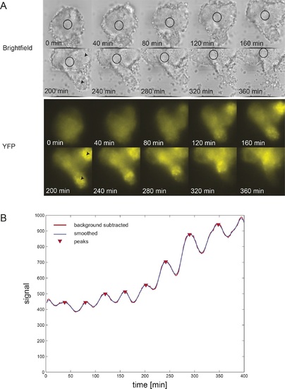
Persistent oscillations in explanted tailbud.(A) Montage of brightfield and corresponding YFP images from representative explanted tailbud over ~7 hr recording. Brightfield image is a single z-plane, while YFP signal is shown as an average projection of the entire stack. Oscillations in the tailbud were measured using a region of interest (ROI; black circle) to extract average YFP intensity values over time. We placed this region on the most central “tailbud” area, as we observed “PSM”-like protrusions (black arrowheads) emerging from the explant. These areas, as expected for PSM, showed brighter and increasing YFP expression over time, which then switched off. (B) Intensity over time plot for the ROI shown in A. The tailbud area shows 9 cycles over the recording with no slowing of the period. Peak finding was performed as in Figure 1-figure supplement 2: background subtracted raw data (thick red line) was smoothed (thin blue line) and peaks were identified (red down triangles). |

Characterization of Ntla and Tbx16 antibodies. (A, D) Graphical representation of the full-length Ntla and Tbx16 proteins with exons depicted in different colors. Blue arrows show the predicted T-box domain from amino acid 35 to 212, and 31 to 213, for Ntla and Tbx16 respectively. The Ntla antibody (clone D18-4, IgG1) was generated using a peptide from amino acid 1 to 261, while the corresponding sequence for the Tbx16 antibody (clone C24-1, IgG2a) spans the region from amino acid 232 to 405 (bracketed in red in both cases). (B, E) Representative examples showing ntla mRNA and protein expression patterns in wild type and in ntla mutant embryos at 90% epiboly. Immunolabeling using the Ntla antibody was followed by in situ hybridization using a ntla riboprobe. The same procedure was used to characterize the Tbx16 antibody except that wild type embryos are compared to tbx16 morpholino-injected embryos and a tbx16 riboprobe was used. Scale bar = 150 µm. (C, F) Immunolabeling of wild type embryos injected at 1-cell-stage with capped mRNAs (Ntla-T2A-mKate2CAAX, Tbx6-T2AmKate2CAAX, Tbx6l-T2A-mKate2CAAX or Tbx16-T2A-mKate2CAAX), fixed at 4 hr post fertilization and imaged at the animal pole where the endogenous genes are not expressed. Both Ntla (C) and Tbx16 (F) antibodies bind only in embryos injected with ntla and tbx16 mRNA respectively, demonstrating antibody specificity. Scale bar = 20 µm. |
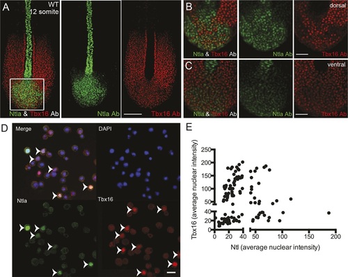
Expression of tailbud markers in vivo and in low-density cultures of segmentation clock cells.(A) z-stack projection showing the expression patterns of Ntla (green) and Tbx16 (red) protein in a 12-somite stage wild type embryo detected using immunohistochemistry with monoclonal antibodies D18-4 (IgG1) to Ntla and C24-1 (IgG2a) to Tbx16. Scale bar = 120 µm (B-C) Close up view of the boxed area in (A) showing a single confocal section at dorsal (B) and ventral (C) locations in the tailbud. Scale bar = 60 µm. (D) Representative panels showing expression of Ntla (green) and Tbx16 (red) in single cells within low-density tailbud cultures (serum + Fgf8b) after 5 hr in vitro. Nuclei are labeled with DAPI (blue). Cells single-positive for Ntla and Tbx16 are visible, as are cells co-expressing both proteins. Scale bar = 20 µm. (E) Quantification of nuclear fluorescence intensity of experiment in (D) showing populations of Ntla-positive, Tbx16-positive, and Ntla/Tbx16 co-expressing cells. |